
by Kashif Javaid
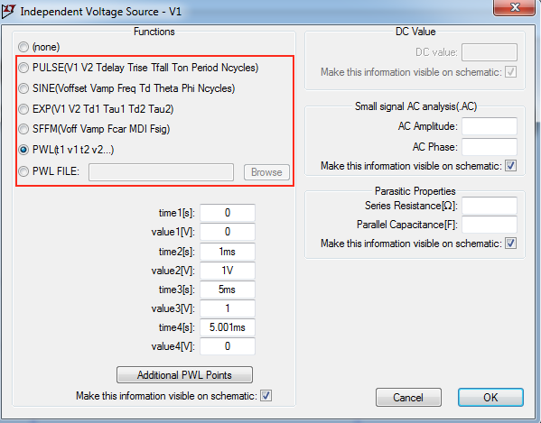
Piece-wise linear voltage or current source is very interesting and can be used to create arbitrary waveforms. Basically you define points (tx, vx) to draw out the precise waveform. For times before t1, the voltage is v1. For times between t1 and t2, the voltage varies linearly between v1 and v2. There can be any number of time, voltage points given. For times after the last time, the voltage is the last voltage as shown below in the dialog box:
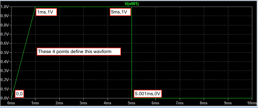
Following waveform is generated with only 4 points.
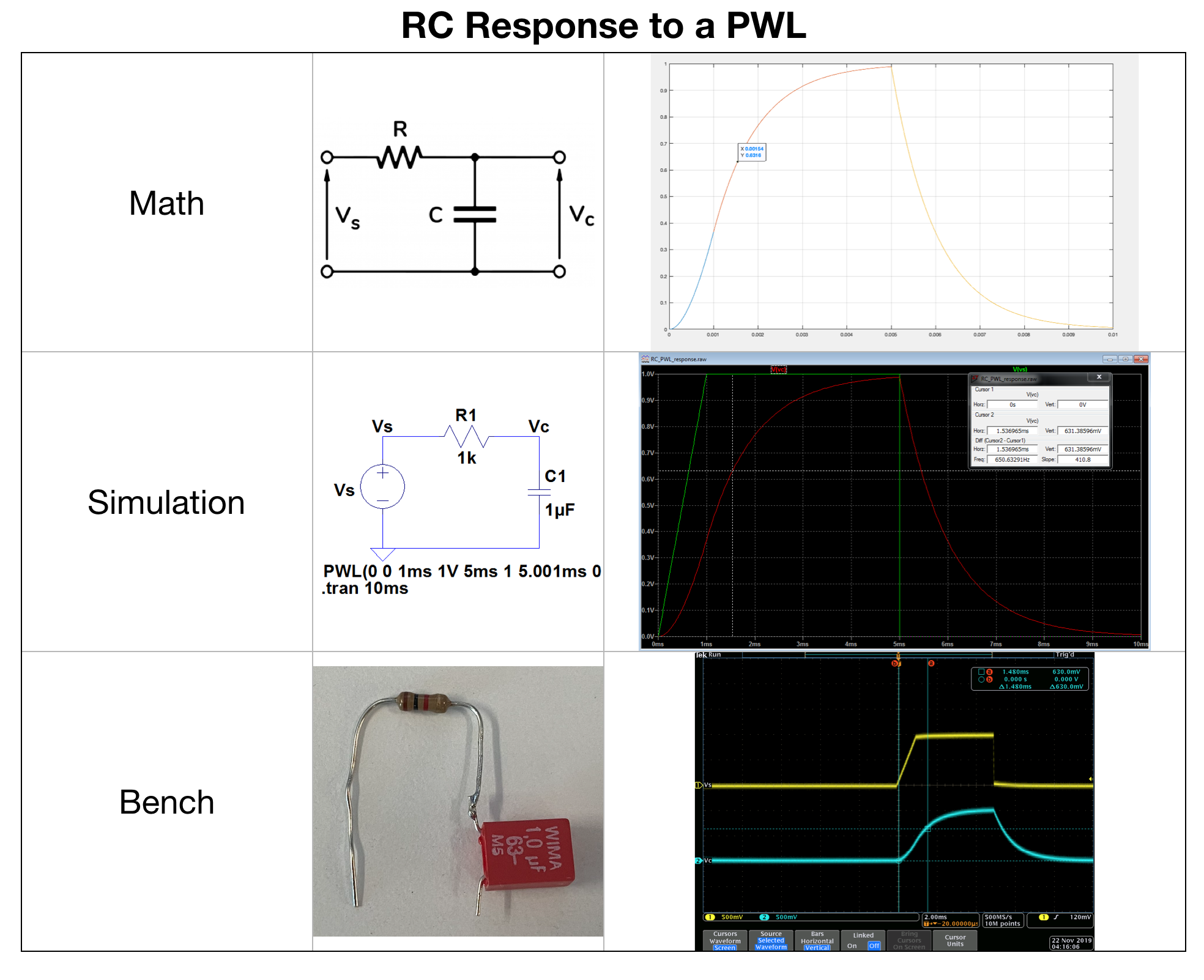
We will use this waveform as a stimulus to same RC circuit. I don’t have a good intuition how the output will look like but I expect this to rise to the final value of 1V but rise ramp will look different than exponential as we are dealing with the ramp. Since this is a simple circuit, we can do some hardcore convolution math to find the formula and plot it in Matlab and then compare it with LTspice to get some confident on the result. Moreover, this stimulus can be easily generated with a typical arbitrary function generator and can be used to get bench result.
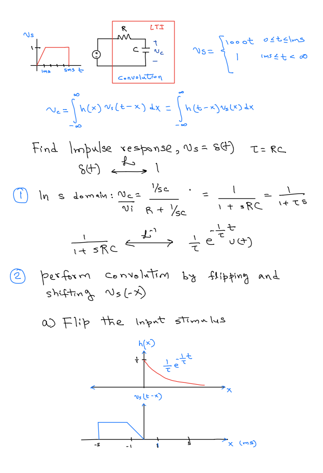
Convolution math can be a bit hairy, but intuition behind it is relative straightforward. First of all convolution formula only apply to Linear Time Invariant or LTI system. This means, once we know the output response called impulse response h(t) from the delta function, an output of any shifted delta function can be found by just shifting the h(t).
A continuous time input can be broken down to bunch of impulses shifted in time. For each of the impulse, output can be determine for a given time and final response will be sum of all the shifted impulse responses. This procedure is illustrated in appendix below for a simple RC circuit. Actually not so simple if input is other than sinusoid or pulse.
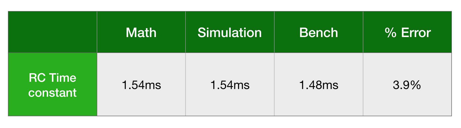
Calculation and simulation results are shown below and RC time constant (not a good parameter for this type of stimulus, but give a number to compare) matches very well. I also got this setup on the bench and actual oscilloscope shot is given. The results and shape of the output curves have excellent agreements.
The calculation/simulation vs bench rc time constant given below:
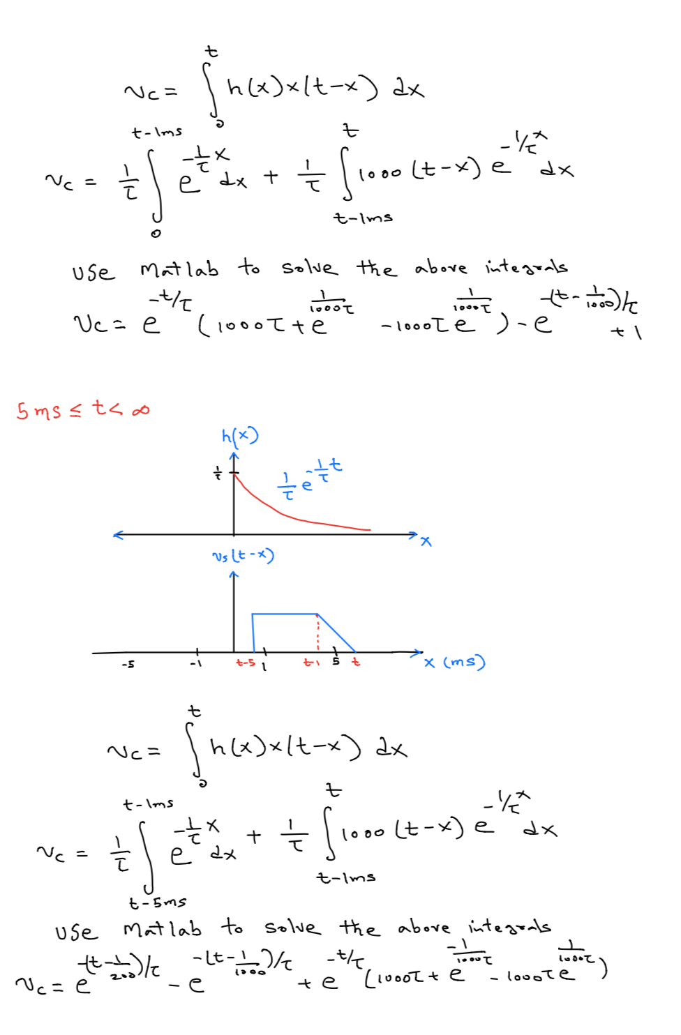
Now the hairy convolution math if you care:

In conclusion, the whole point of this post was to illustrate and build confidence on the LTspice PWL input capability using an example circuit for which we can calculate the exact response.
Download PWL
