Commands covered: .ac .meas 

What is impedance? Impedance is simply defined as voltage divided by current (Z = V/I). This definition of impedance applies to both in the time domain or the frequency domain. In the frequency domain it’s really the magnitude and phase of sine wave that are used for voltage and current. The math involve complex algebra, but doable for simple circuits. This is really the basis to do simulation in LTspice.

V = Z * I

Choose I=1A constant current source, then V = Z. We can measure voltage easily in LTspice that essentially equal to impedance. Let’s illustrate how this work in LTspice using basic passive components.

Figure 1: Simulation circuit for a resistor, a capacitor and an inductor

We expect resistor impedance, normally called resistance, to constant across frequency. For capacitor and inductor we expect impedance to linearly decrease or increase respectively with frequency in log-log plot per following equations:

Z_R = R

Z_C = 1/j(2*pi*f*C)

Z_L = j*2*pi*L

Note complex number j encodes phase information.

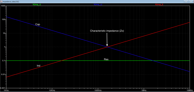
Figure 2: Impedance response of 100mΩ resistor, 1µF capacitor, 1µH inductor

Few points to note:

1. .ac command is used to plot 10kHz to 10MHz with 100 point/decade
2. R2, R5 and R6 are optional, it some version of SPICE, a DC point need to be calculated first. If there is no DC path, simulation will fail. It is a good idea to keep this resistor.
3. V(Imp_X) where X=R or C or R either a voltage in V or impedance in Ω.

Now what about the phase? Glad you asked as it can also be easily plotted—launching the Right Vertical Axis dialog box by clicking on the right axis.

Figure 3: Phase is shown in dashed lines for 100mΩ resistor, 1µF capacitor, 1µH inductor

Typically impedance profile do not show the phase because by knowing the amplitude behavior we know how the phase behaves. If impedance increases (20dB/decade) phase is close to 90˚. If impedance decrease (-20dB/decade), phase is close to -90˚. For the flat impedance, phase 0˚. This is shown in the above plot.

In the next two examples, let’s take a look at the series RLC and the parallel RLC circuits.

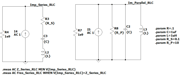
Figure 4: Simulation Circuits for Series and parallel RLC 

For series RLC circuit, let’s intuitively guess the overall impedance. At low and high frequency capacitor and inductor has high impedances, so total impedance should be high at low and high frequencies respectivily. At some point in frequency sweep, the complex impedance of inductor will cancel with the negative complex impedance of capacitor. Since R is constant and will remain, so this will determine the lowest point of impedance. There are four main parameters of a RLC circuit:

1. Resonant Frequency: Fres = 1 / (2*pi*sqrt(L*C)
2. Characteristic impedance = Zo = sqrt(L/C)
3. Quality Factor: Q = Zo / R
4. Zmin = R = Zo / Q

For our chosen values R=100mΩ, C=1µF, L=1µH, Fres = 159kHz, Zo=1, Zmin=100mΩ, Q=10.

It’s easy to measure resonant frequency in LTspice using cursor or .meas statement. The spice error log file from View show:

z_series_rlc: MIN(v(imp_series_rlc))=(-19.9136dB,0.0780292°) FROM 1000 TO 1e+007

fres_series_rlc: v(imp_series_rlc)=z_series_rlc AT 159166

I used two .meas statements to calculate resonant frequency. First I calculated the min impedance value. Using this value to find resonant value on frequency axis (see the .meas statements in figure 4.

Characteristic impedance is a crossover point where capacitor’s impedance is equal to inductor’s impedance. This can be seen in the plot below. The value of characteristic impedance directly determine the quality factor, relative sharpness of the peak in impedance profile.

For parallel circuit, only thing change is the definition of Q = R / Zo. In Parallel RLC case, Zmax = R = Q*Zo. This can clearly be seen in the following plot. Note, Zo is the same in both cases and how the Q gives the indication of “peaking” in impedance. Feel free to download this .asc file and play with it to get deeper understanding of all the parameters involved.

Figure 5: Impedance response of Series and Parallel  RLC circuit 

Download examples here:

Discuss this topic here:

https://www.eevblog.com/forum/projects/ltspice-lesson-5-how-to-simulate-impedances/msg3132552/#msg3132552